Microsoft Excel is a powerful spreadsheet software. I have a student report sheet in MS-Excel. There are three columns in this sheet.
Column A : Name of the students
Column B : Marks Obtained
Column C : Grade
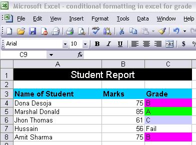
Column A and Column B are the inputs by the user and Column C is grade of the students that is depend on following four criteria:
1. if obtained marks are more than or equals to 80 and less than 90 grade would be "A"
2. if obtained marks are more than or equals to 70 and less than 80 then grade would be "B"
3. if obtained marks are more than or equals to 60 and less than 70 then grade would be "C"
4. if obtained marks are less than 60 then grade would be "Failed"
For above purpose put this "IF" function in C4 column
The function is =IF(B4>=80,"A",IF(B4>=70,"B",IF(B4>=60,"C","Failed")))
and then copy this function to all the required cells.
Now I need some conditional formatting on column C for the following criteria:
a. If marks are greater than or equals to 80 and less than 90 then background color of the cell should be green
b. If marks are greater than or equals to 70 and less than 80 then background color of the cell should be purple
c. If marks are greater than or equals to 60 and less than 70 then background color of the cell should be gray
To achieve this follow the step by step process:
Step 1: Select the cells of C column (Grade) where conditional formatting to be applied.
Step 2: then click Format Menu.
Step 3: then choose Conditional Formatting.. From the menu.
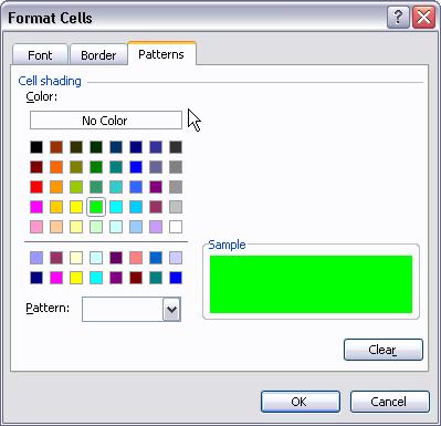
Step 4: Conditional formatting dialogue box will be appeared on the screen. Under condition 1 choose Formula Is from the drop down menu and then type this formula in the text box.


=AND(IF(B4>=80,B4<90))
Step 5: then click Format button to assign formatting.
Step 6: Format cells dialogue box will be appeared on the screen. Click Patterns tab on the window and then choose desired color. In our case we will select green color and then press Ok button.
Step 7: Now press Add button to add second conditional formatting condition.
Step 8: Repeat the Step 4 to 6 for the next 2 conditions and assign their different formula and colors.
We can assign total three conditions for conditional formatting.
Now try with different marks, when you change marks, according to the marks background color of the cell will be changed.


No comments:
Post a Comment